Secrets of Time Series Forecasting & its Statistical Nuances

A time series is a collection of data points gathered over time that can be used to analyse & forecast trends and patterns. Working with time series data requires caution because one wrong step can lead to misleading results. The three things to consider when working with time series data are as follows:

Spurious Correlation:
When we have two time series datasets that are highly dependent on the passage of time. Examples include stock market index data over time and the number of goals scored by a footballer over time. Because the factors are highly dependent on time, the values for both datasets are bound to rise in the long run, say 5-6 years. If you calculate the correlation between them, you'll find that it's extremely positive. However, this does not imply that the variables, stock market data and football goals, are in any way related. The increase in values is due to the passage of time, which results in a positive correlation. Because there is ultimately no casual relationship between them, we are unable to determine if they are related in any manner or not. There is no link of any type between stock market data and a football player's goals scored.

Series or Order of Data:
The word "series" is used in Time Series for a specific reason. The reason is that while working with time series, the order of the data is crucial. We cannot randomly shuffle the data and take out a fragment of data to perform our analysis on it.  The order of the data is critical, and we must take it seriously. We must be extra cautious when performing any training/test or cross validation because these steps require some form of series shuffling, which somehow diminishes the core concept behind the series.

Duration of Data:
Consider a scenario in which you want to perform some sort of time series forecasting. You might be tempted to do this with only a few years' worth of data. But keep in mind that you will need at least three to four years of data to perform any kind of reasonable time series forecasting because only if you have that much data, you will be able to observe seasonality.

Let’s understand what this term seasonality means. Seasonality in time series refers to the presence of repeating patterns over a set period of time. These patterns may be impacted by regular occurrences such as the season or holidays; Seasonality can be seen in a variety of time series data, including product sales, website traffic, and weather patterns. These patterns can have a substantial impact on how data is interpreted and the accuracy of forecasts.

We have to be careful not only in using data for a shorter period but also be very careful while using the data of 7 or 8 years. The reason to be extra cautious in a longer period is the structural breaks which could happen in the long run.  A structural break in a time series refers to a significant modification of the method used to produce the data, such as a sudden change in trend or a modification in the correlation between variables. Time series data analysis and forecasting may be significantly impacted by these breaks. 

These above 3 points must be considered to improve your time series analysis forecasting.

The problem with pooled data - Simpson's Paradox - Grouped Data

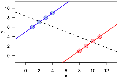
Simpson's Paradox occurs when the direction or strength of an association between two variables changes when data is divided into subgroups. In 1951, statistician Edward Simpson described the paradox for the first time. When data is split, a trend or relationship that was observed in a group of data points disappears or reverses. 

Let’s understand Simpson’s Paradox by an example. Assume a university is comparing the admission rates of male and female applicants over the last five years. The overall admission rate is 54%, but when the data is broken down by gender, the admission rate for male applicants is 70%, while it is only 50% for female applicants.

All		Male		Female
Applicants	Admitted	Applicants	Admitted	Applicants	Admitted
1000	54%	650	70%	350	50%

When there is a confounding variable that is related to both the independent and dependent variables, this dilemma occurs. Confounding variable means an extraneous variable which is correlated with both dependent and independent variables. The confounding variable in this example is the department to which the applicants are applying. Male candidates predominate in departments with greater acceptance rates, while female applicants predominate in departments with lower admission rates. As a result, when the data is pooled across all departments, male candidates appear to have a greater admission rate than female applicants.

Department	All		Male		Female
	Applicants	Admitted	Applicants	Admitted	Applicants	Admitted
A	250	31%	90	38%	160	34%
B	290	42%	180	48%	110	42%
C	460	75%	380	85%	80	81%

The examination of medical therapies is another example of Simpson's Paradox. Assume a new medicine is being tested for its efficacy in treating a specific condition. In a clinical trial, the medicine was shown to be successful in the majority of patients, with 80% showing improvement. However, when the data is broken down by age, it is discovered that the medicine is only helpful for those over the age of 60. This paradox emerges because the patients' age is a confounding element that influences the link between treatment and illness improvement.

To prevent Simpson's Paradox, it is critical to identify and analyse relevant confounding variables. One method is to stratify the data by the confounding variable and study each subgroup individually. In the case of university admissions, stratifying the data by department reveals the true relationship between gender and admission rate. Another option is to control for the confounding variable using regression analysis. This can help to determine the true relationship between the independent and dependent variables.

For making decisions and creating policies, Simpson's Paradox has serious repercussions.  It implies that more detailed data analysis is necessary because aggregate data can be misleading. It might not be ethical to recommend a medical procedure to all patients, for instance, if a clinical trial reveals that it is successful but later research reveals that it only works for a particular subgroup of patients. 

In summary, Simpson's Paradox is a statistical phenomenon that can happen in the presence of a confounding variable. If data are only examined at an aggregate level, it may result in false conclusions. It is necessary to recognise potential confounding variables and analyse them appropriately, either by stratifying the data or by using regression analysis, in order to avoid Simpson's Paradox. Making informed decisions and developing effective policies based on data analysis require an understanding of Simpson's Paradox.